Chargement OSM données dans GeoNode¶

Dans cette section, nous allons marcher à travers les étapes nécessaires pour charger les données OSM dans votre projet de GeoNode. Comme indiqué dans les sections précédentes, votre GeoNode utilise déjà tuiles OSM de MapQuest et les principaux serveurs de l’OSM que quelques-unes des couches de base disponibles. Cette session est spécifiquement sur l’extraction de données réelles de l’OSM et de conversion pour l’utiliser dans votre projet et potentiellement pour des tâches de géotraitement.

La première étape de ce processus est d’obtenir les données de l’OSM. Nous allons utiliser l’API OSM Overpass car il nous permet de faire des requêtes plus complexes que l’API OSM lui-même. Vous devez vous référer à la documentation de l’API OSM viaduc pour en apprendre davantage sur l’ensemble de ses fonctionnalités. Il est une API extrêmement puissant qui vous permet d’extraire les données de l’OSM en utilisant une API très sophistiqué.

In this example, we will see a couple of examples extracting:

Southwest Platte River Road footprint, which runs through Denver

Building footprint data around Kampala, Uganda.

To do this we will use an interactive tool that makes it easy construct a Query against the Overpass API.

Exportation des données OSM à ShapeFile utilisation de QGIS¶

First go to openstreetmap.org, and search for “South Platte River, Denver”

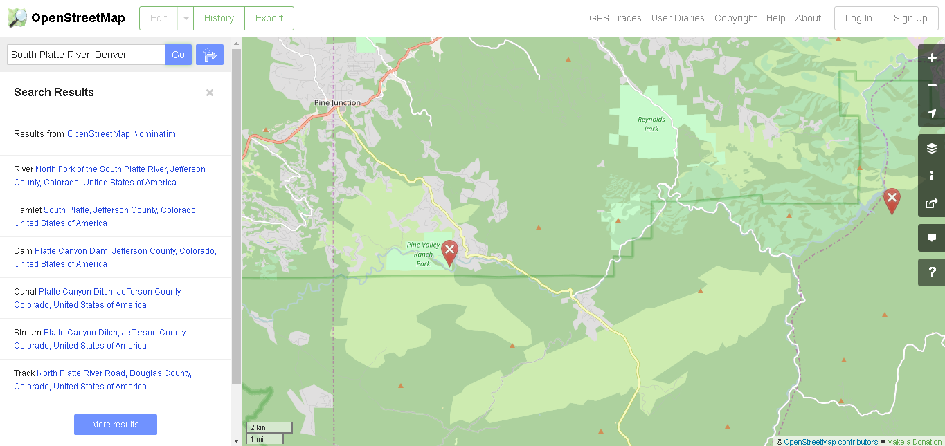
Search on OpenStreetMap
Zoom in, until you see the features appearing

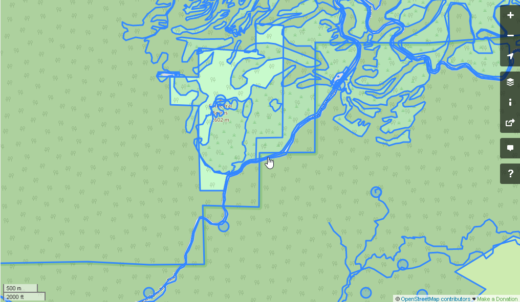
Features on OpenStreetMap
Select a feature. In this example we selected Way: Southwest Platte River Road (17082695)

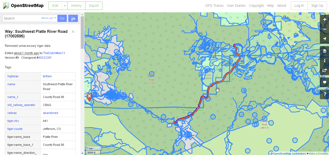
Southwest Platte River Road
Identify the tags and values of the features you’re after by
- Zooming all the way into the map
- Click on the layers icon on the right (the three sheets of paper)
- Click on the last menu entry (Map data or something similar in your language)
- The features on the map turn blue (make sure you’re zoomed in far enough to see
- Click on the feature you’re after
- The Tags and Values appear on left side of the screen, and you can proceed below...
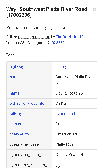
Southwest Platte River Road - Details
Point your browser at overpass-turbo.eu, and use the search box to zoom to the area of interest, in this case Colorado

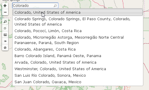
Colorado
Click on the Wizard button, and enter the search text accordingly to the information retrieved from OpenStreetMap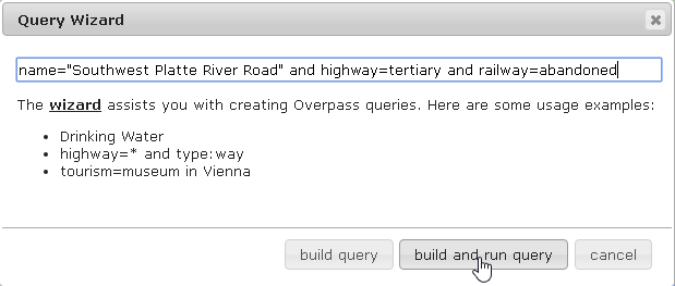
Southwest Platte River Road
name="Southwest Platte River Road" and highway=tertiary and railway=abandoned
Click on the button Build and Run Query, the map shows the selected data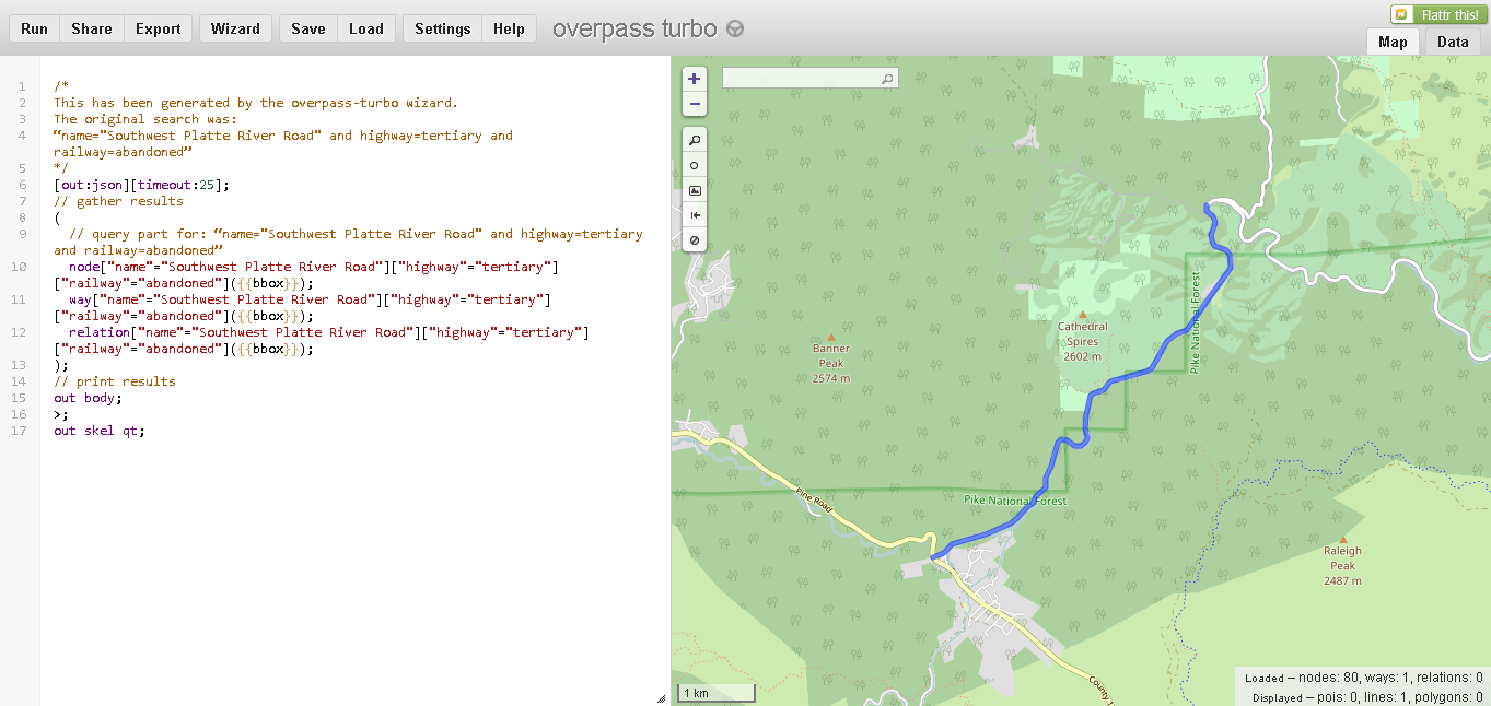

Southwest Platte River Road Data
Click on the button Export, and download data as GeoJSON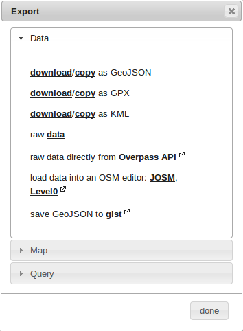

Southwest Platte River Road Export
Save it and confirm. The file export.geojson will be created into the Downloads folder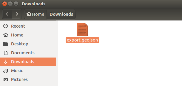

export.geojson
Rename the file to south_platte_river_road.geojson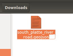

south_platte_river_road.geojson
Open QGis Client and import the layer into it

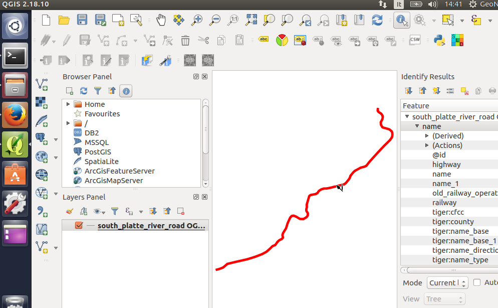
QGis Client
Click with the right button over the layer and then click on Save As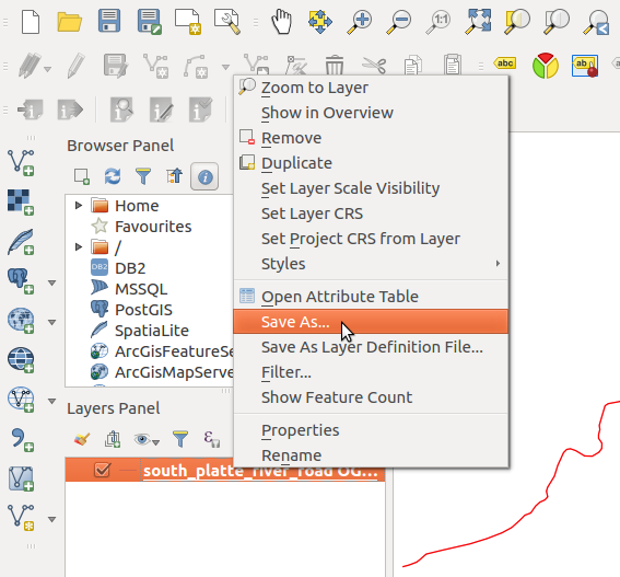

QGis Client - Save As
Select ESRI Shapefile and click on Browse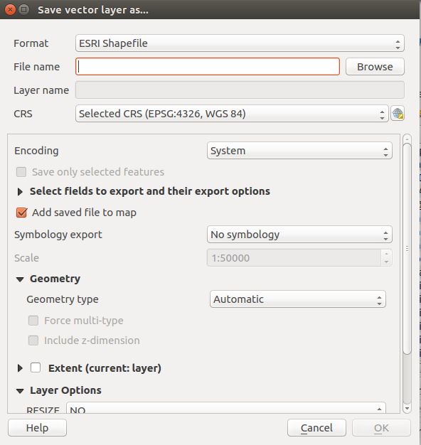

QGis Client - Save As SHP
Select the Downloads folder and name the file south_platte_river_road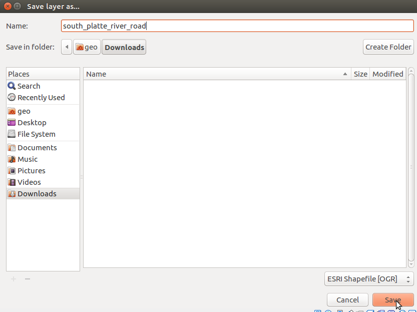

QGis Client - Save As SHP
This will save the layer as a Shapefile, which can be easily imported into GeoNode

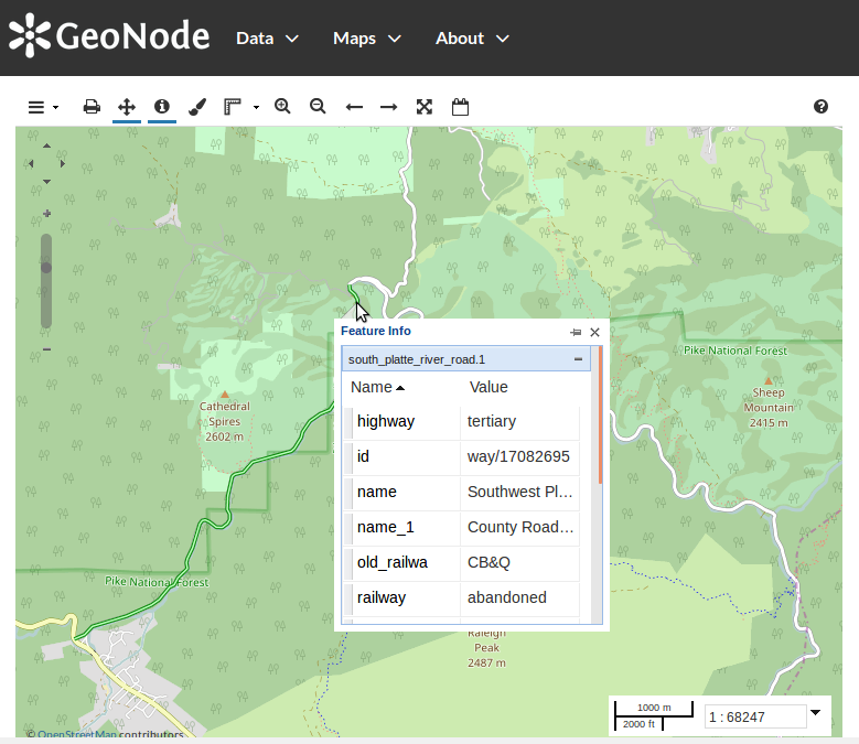
South Platte River Road into GeoNode

Let’s see another example of export through the OverPass APIs.

Point your browser at overpass-turbo.eu, and use the search box to zoom to the area of interest, in this case Kampala

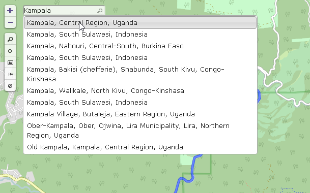
Kampala
Zoom around Nakasero area

Nakasero
Select the desired Bounding Box around the area to export

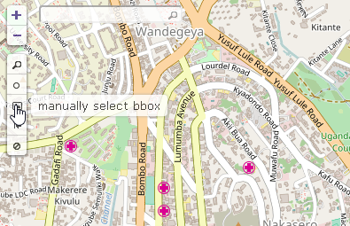
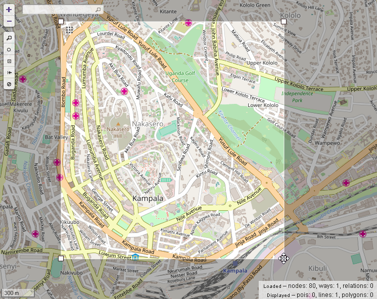
Nakasero BBOX

Run the Wizard and write building=* or highway=* in bbox on the text box.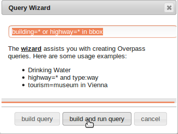

Nakasero Query Builder

This will result in a query like the following one

/*
This has been generated by the overpass-turbo wizard.
The original search was:
“building=* or highway=* in bbox”
*/
[out:json][timeout:25];
// gather results
(
  // query part for: “building=*”
  node["building"]({{bbox}});
  way["building"]({{bbox}});
  relation["building"]({{bbox}});
  // query part for: “highway=*”
  node["highway"]({{bbox}});
  way["highway"]({{bbox}});
  relation["highway"]({{bbox}});
);
// print results
out body;
>;
out skel qt;

Export data as GeoJSON like before, rename it and use QGis to export as a Shapefile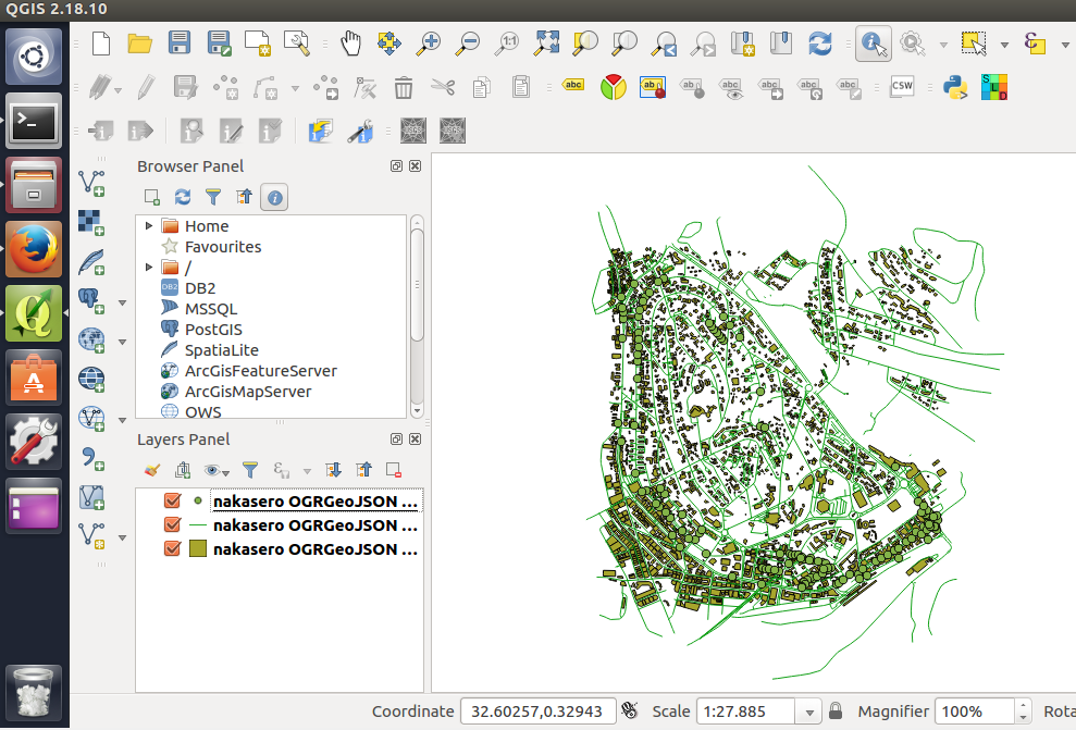

Nakasero Query Builder
This will allow you to save all the layers as a Shapefiles, which can be easily imported into GeoNode

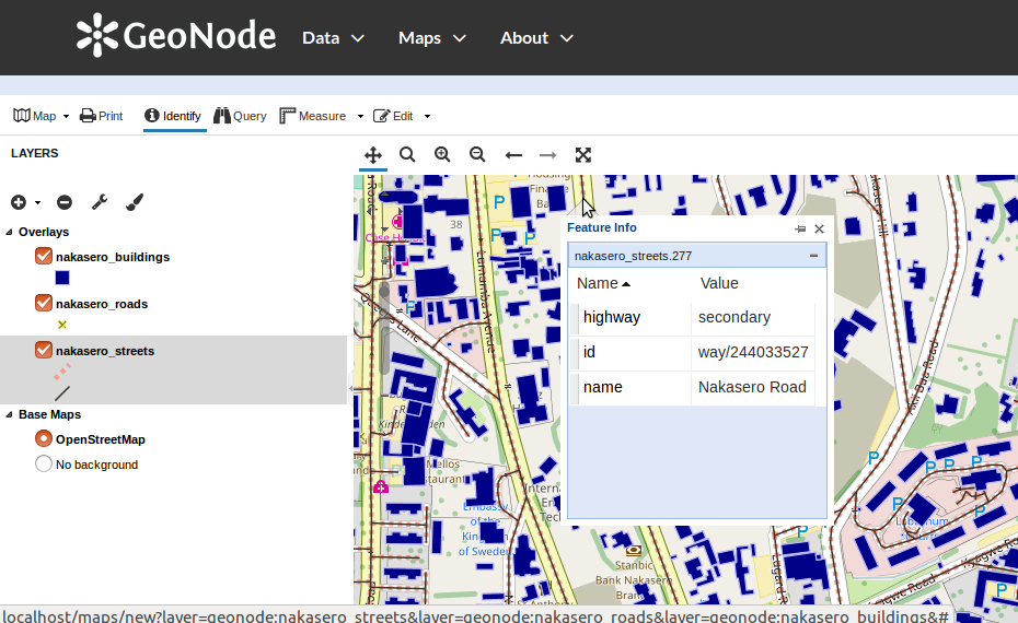
Nakasero into GeoNode

Note

Vous pouvez également renommer le fichier dans votre exploitation outil de gestion des systèmes de fichiers (Windows Explorer, Finder, etc.).

Note

Vous voudrez peut-être passer à une couche d’imagerie afin de voir plus facilement les bâtiments sur le fond de l’OSM.

Exportation des données OSM à ShapeFile utilisant GDAL¶

An alternative way to export the .osm or .geojson file to a shapefile is to use ogr2ogr combined with the GDAL osm driver, available from GDAL version 1.10.

Dans un premier temps, inspecter la manière dont le pilote de GDAL OSM voit le fichier .osm aide de la commande ogrinfo

$ ogrinfo -al -so nakasero.geojson -where "OGR_GEOMETRY='Point'"

INFO: Open of `nakasero.geojson'
      using driver `GeoJSON' successful.

Layer name: OGRGeoJSON
Geometry: Unknown (any)
Feature Count: 142
Extent: (32.573864, 0.312602) - (32.593496, 0.331627)
Layer SRS WKT:
GEOGCS["WGS 84",
    DATUM["WGS_1984",
        SPHEROID["WGS 84",6378137,298.257223563,
            AUTHORITY["EPSG","7030"]],
        AUTHORITY["EPSG","6326"]],
    PRIMEM["Greenwich",0,
        AUTHORITY["EPSG","8901"]],
    UNIT["degree",0.0174532925199433,
        AUTHORITY["EPSG","9122"]],
    AUTHORITY["EPSG","4326"]]
id: String (0.0)
...

$ ogrinfo -al -so nakasero.geojson -where "OGR_GEOMETRY='LineString'"

INFO: Open of `nakasero.geojson'
      using driver `GeoJSON' successful.

Layer name: OGRGeoJSON
Geometry: Unknown (any)
Feature Count: 928
Extent: (32.571923, 0.306984) - (32.597590, 0.338549)
Layer SRS WKT:
GEOGCS["WGS 84",
    DATUM["WGS_1984",
        SPHEROID["WGS 84",6378137,298.257223563,
            AUTHORITY["EPSG","7030"]],
        AUTHORITY["EPSG","6326"]],
    PRIMEM["Greenwich",0,
        AUTHORITY["EPSG","8901"]],
    UNIT["degree",0.0174532925199433,
        AUTHORITY["EPSG","9122"]],
    AUTHORITY["EPSG","4326"]]
id: String (0.0)
...

$ ogrinfo -al -so nakasero.geojson -where "OGR_GEOMETRY='Polygon'"

INFO: Open of `nakasero.geojson'
      using driver `GeoJSON' successful.

Layer name: OGRGeoJSON
Geometry: Unknown (any)
Feature Count: 2596
Extent: (32.572918, 0.311164) - (32.594049, 0.333597)
Layer SRS WKT:
GEOGCS["WGS 84",
    DATUM["WGS_1984",
        SPHEROID["WGS 84",6378137,298.257223563,
            AUTHORITY["EPSG","7030"]],
        AUTHORITY["EPSG","6326"]],
    PRIMEM["Greenwich",0,
        AUTHORITY["EPSG","8901"]],
    UNIT["degree",0.0174532925199433,
        AUTHORITY["EPSG","9122"]],
    AUTHORITY["EPSG","4326"]]
id: String (0.0)
...

$ ogrinfo -al -so nakasero.geojson -where "OGR_GEOMETRY='MultiPolygon'"

INFO: Open of `nakasero.geojson'
      using driver `GeoJSON' successful.

Layer name: OGRGeoJSON
Geometry: Unknown (any)
Feature Count: 3
Extent: (32.576421, 0.315224) - (32.590876, 0.330137)
Layer SRS WKT:
GEOGCS["WGS 84",
    DATUM["WGS_1984",
        SPHEROID["WGS 84",6378137,298.257223563,
            AUTHORITY["EPSG","7030"]],
        AUTHORITY["EPSG","6326"]],
    PRIMEM["Greenwich",0,
        AUTHORITY["EPSG","8901"]],
    UNIT["degree",0.0174532925199433,
        AUTHORITY["EPSG","9122"]],
    AUTHORITY["EPSG","4326"]]
id: String (0.0)
...

ogrinfo has detected 4 different geometric layers inside the osm data source. As we are just interested in the buildings, you will just export to a new shapefile the polygons and multipolygons layer using the GDAL ogr2ogr command utility:

$ ogr2ogr nakasero_buildings nakasero.geojson -where "OGR_GEOMETRY='Polygon' or OGR_GEOMETRY='MultiPolygon'" -nln nakasero_buildings

Maintenant, vous pouvez télécharger le fichier de formes GeoNode en utilisant le formulaire GeoNode chargement de la même manière que vous avez fait dans la section précédente.