# Optimizing, publishing and styling GeoTIFF data
## Styling with CSS
The CSS extension module allows to build map styles using a compact, expressive styling language already well known to most web developers: `Cascading Style Sheets`.
The extension is available on GeoServer only. The standard CSS language has been extended to allow for map filtering and managing all the details of a map production. In this section we'll experience creating a few simple styles with the CSS language.
### Styling raster data
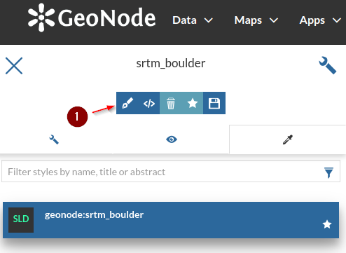
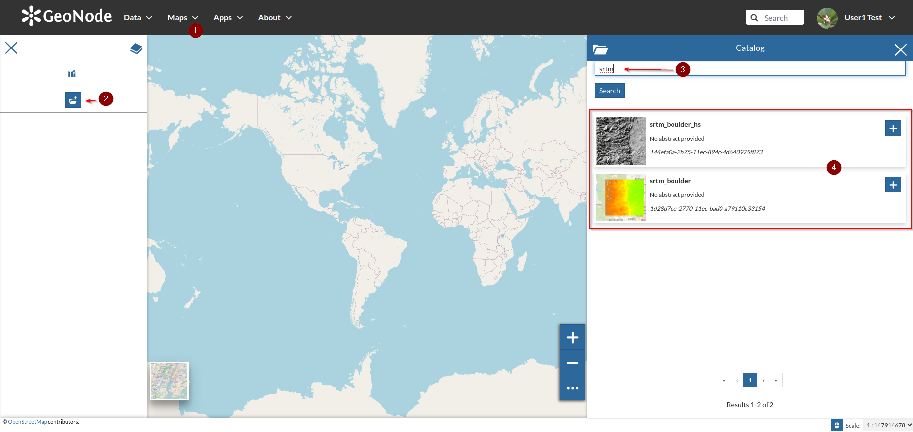
- Go to the `srtm_boulder` layer details page and click on `Editing Tools > Style > Edit`

- Add a new `Style`
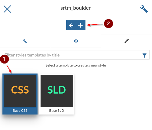
- Select `CSS` and click on the `+` button
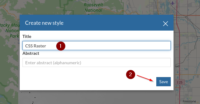
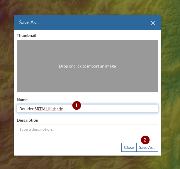
- Put a name like `CSS Raster` and click on `Save`
- Modify the style you just created
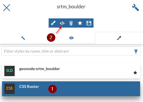
- From the panel, switch to the advanced editor
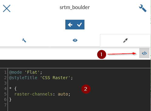
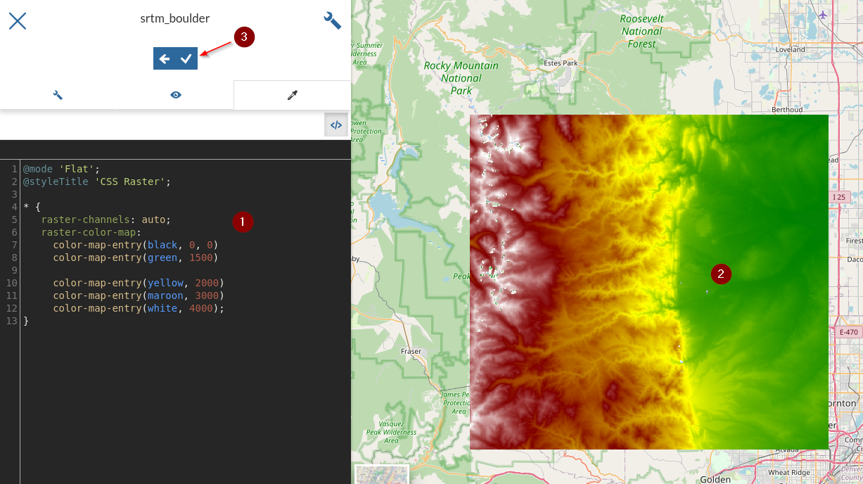
- Insert the following `CSS`, notice the changes directly on the map, and `Save`
```css
* {
raster-channels: auto;
raster-color-map:
color-map-entry(black, 0, 0)
color-map-entry(green, 1500)
color-map-entry(yellow, 2000)
color-map-entry(maroon, 3000)
color-map-entry(white, 4000);
}
```
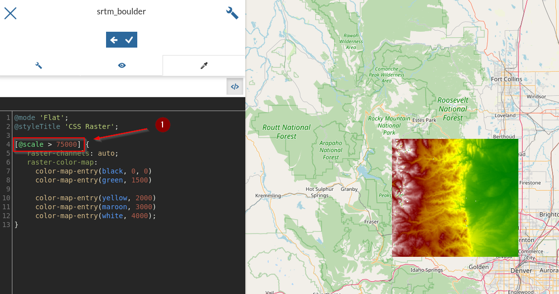
- The `*` at the beginning means that we will apply the rules at any zoom level; let's add a rule to show the raster only above a certain `scale denominator`
```css
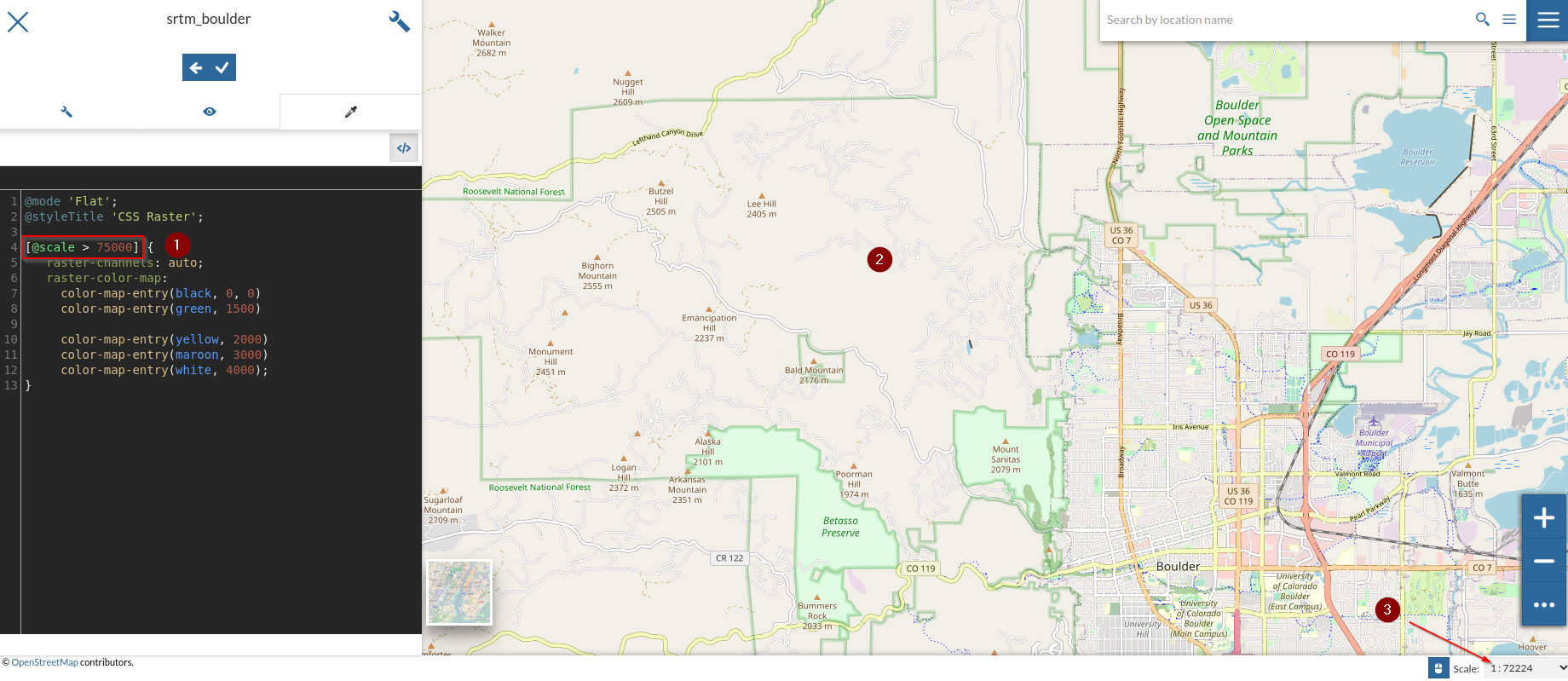
[@scale > 75000] {
raster-channels: auto;
raster-color-map:
color-map-entry(black, 0, 0)
color-map-entry(green, 1500)
color-map-entry(yellow, 2000)
color-map-entry(maroon, 3000)
color-map-entry(white, 4000);
}
```
- Try to zoom in and out by checking the `scale denominator`; notice the raster appearing and disappearing accordingly
## Nice Map with Hillshading
In this section we are going to create a `hillshade` raster computed from the `srtm DEM` of Boulder. We will use the `GDAL` utilities to do that, and in particular the `gdaldem` one, which has several options available.
Once we created the `hillshade`, we will add it to GeoNode, provide a nice style and then merge all together on a nice map.
- Go to the `terminal` and move to the folder `/opt/data/sample_data/pretty_maps/data/boulder/`
- Run the `gdaldem` utility with the following options
```shell
gdaldem hillshade -z 5 -s 111120 srtm_boulder.tiff srtm_boulder_hs.tiff -co tiled=yes
```
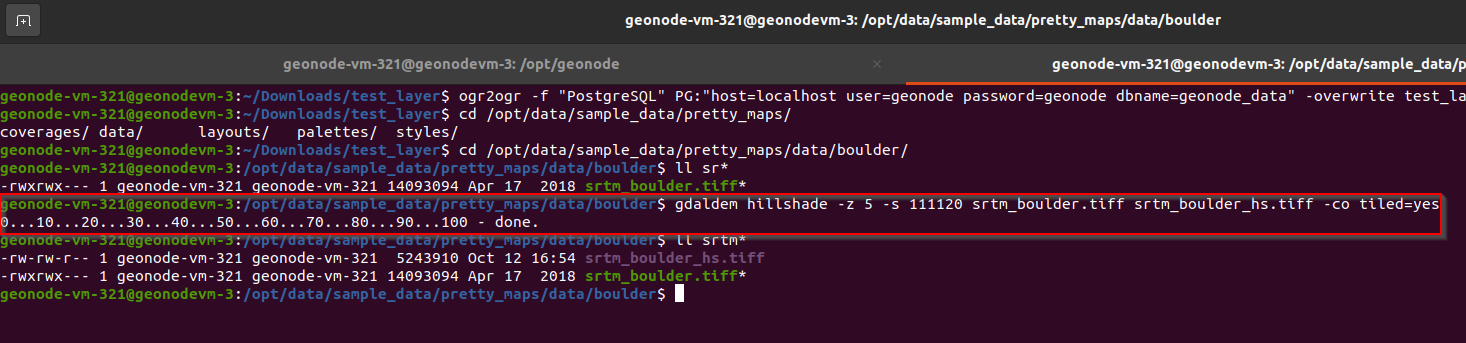
_The z parameter exaggerates the elevation, the s parameter provides the ratio between the elevation units and the ground units (degrees in this case), -co tiled=yes makes gdaldem generate a TIFF with inner tiling. We’ll investigate this last option better in the following pages._
- That will create a new `GeoTIFF` called `srtm_boulder_hs.tiff`
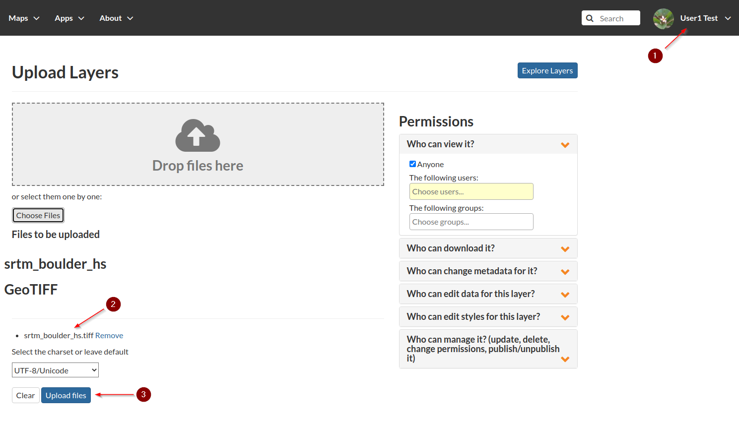
- Upload the new layer as user `test_user1`
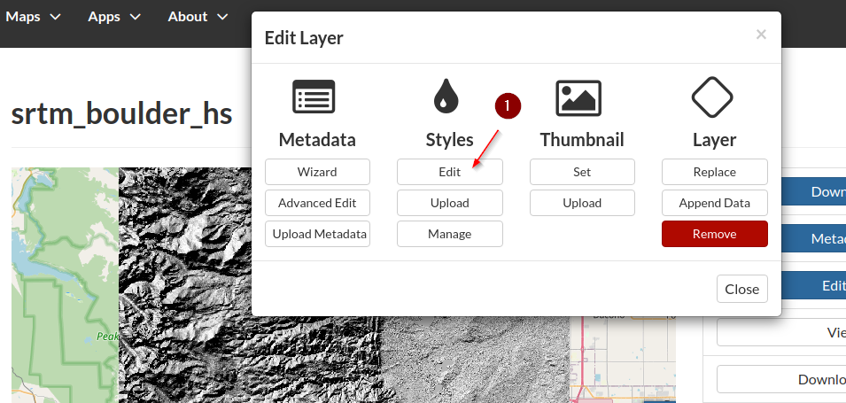
- Edit the style for this layer too; a new `CSS` named `Hillshade CSS`
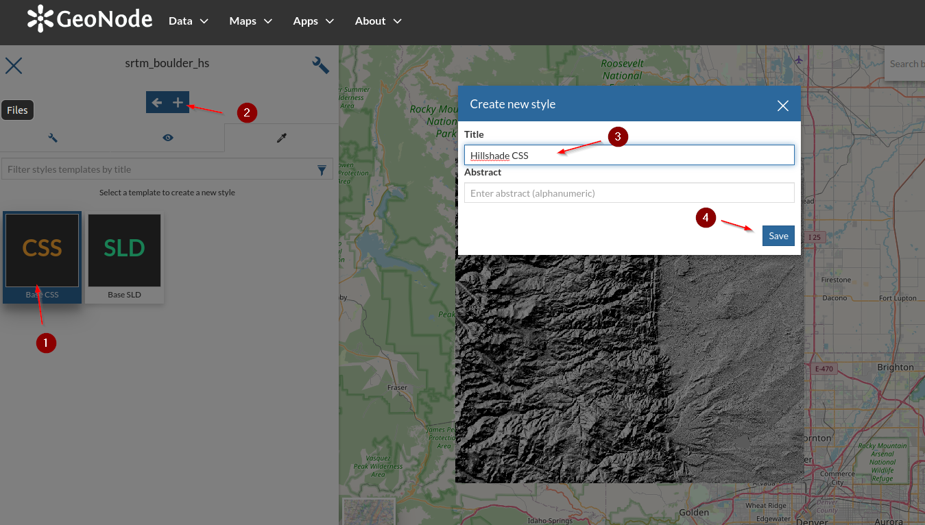
- Insert the `CSS` below and save
```css
[@scale > 75000] {
raster-channels: auto;
raster-color-map:
color-map-entry(#000000, 0, 0)
color-map-entry(#999999, 1)
color-map-entry(#FFFFFF, 256);
composite: 'multiply';
}
```
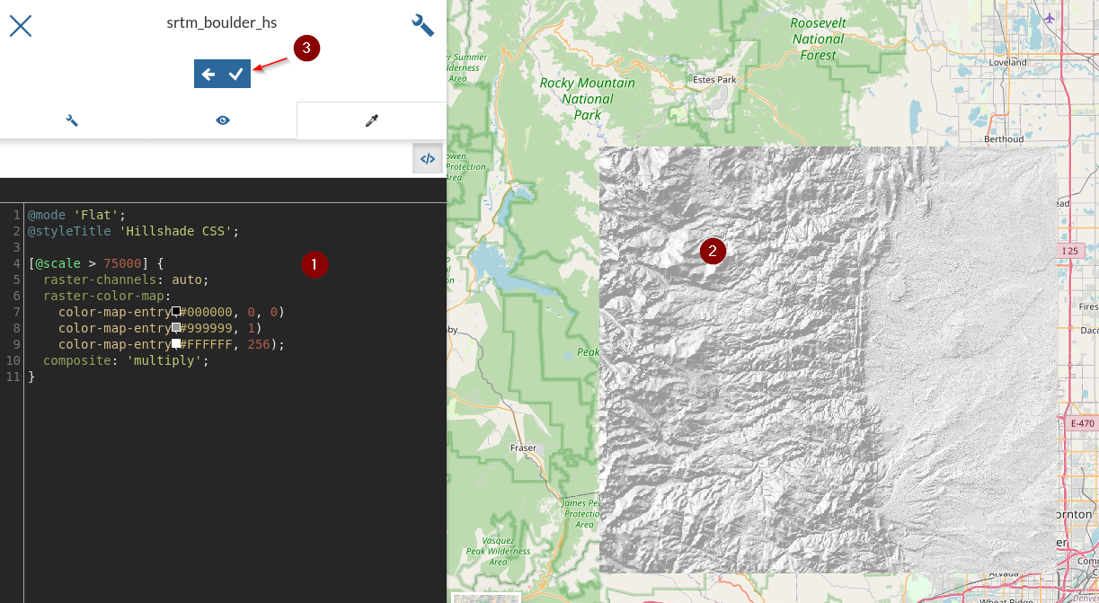
_Note the “composite” vendor option, used to have the hillshading use a special color blending mode to get a better visual result compared to simple translucency_
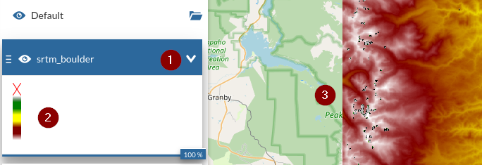
- Create a new `Map` and add the two raster layers just updated
- Highlight the `srtm_boulder` and the `modify` option
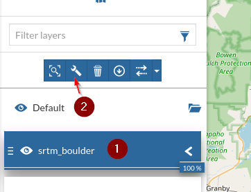
- Select the `style` tab, click on the `CSS Raster` style and `Save`
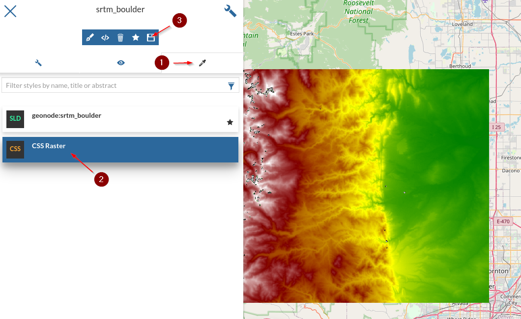
- Notice the `legend` has changed and so the rendering on the map for that layer
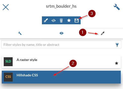
- Similarly go ahead and select the `Hillshade CSS` for the `srtm_boulder_hs` layer
- Adjust the overlays `order` and `opacity` and notice the map changing accordingly
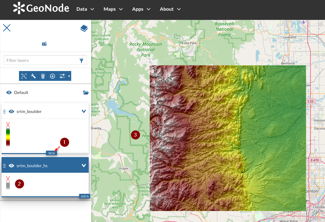
- Zoom-in in order to highlight the details and the color effect enhanced by the hillshade
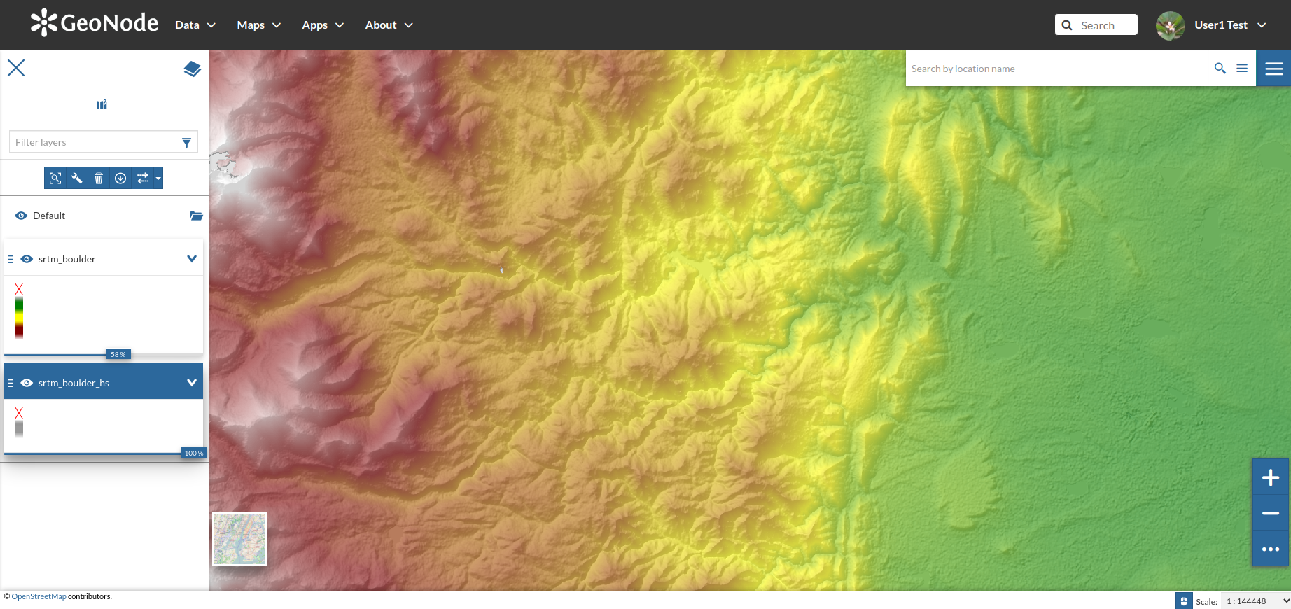
- Save the new map when done
## Adding and Optimizing Raster Image Mosaics
An `Image Mosaic` is composed of a set of `layers` which are exposed as a `single coverage`. The `ImageMosaic` format allows to **automatically** build and setup a mosaic from a set of `georeferenced layers`. This section provides better instructions to configure an `Image Mosaic`.
### Publishing an Image Mosaic
In this section we are going to publish on GeoNode a `mosaic` of aerial `orthophotos` through the GeoServer `ImageMosaic` store.
We will need to do some preparation first.
- Open a `terminal` and move to the folder `/opt/data/sample_data/user_data`; change the `write` permissions of the folder named `aerial` in order to allow the user to modify it
```shell
cd /opt/data/sample_data/user_data
sudo chmod -Rf 777 aerial
```
- Move to `aerial` and delete the files `aerial.properties` and `sample_image.dat`
```shell
cd aerial
rm aerial.properties sample_image.dat
```
- Create or edit a file named `indexer.properties` with the following contents
```shell
vim indexer.properties
```
```ini
Caching=false
Schema=*the_geom:Polygon,location:String
```
- Create or edit a file named `datastore.properties` with the following contents
```shell
vim datastore.properties
```
```ini
SPI=org.geotools.data.postgis.PostgisNGDataStoreFactory
host=localhost
port=5432
database=geonode_data
schema=public
user=geonode
passwd=geonode
Loose\ bbox=true
Estimated\ extends=false
validate\ connections=true
Connection\ timeout=10
preparedStatements=true
create\ database\ params=WITH\ TEMPLATE\=postgis20
```
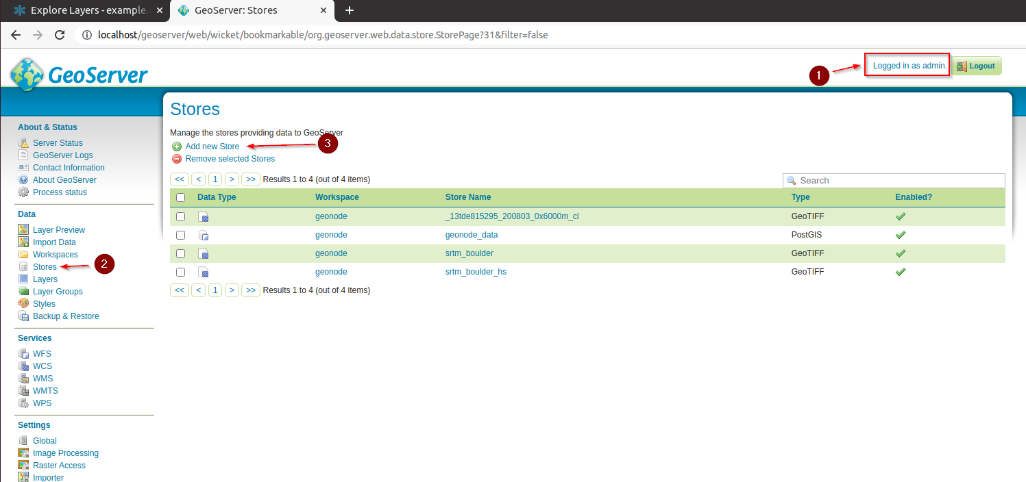
- Go to the GeoServer admin dahsboard; log in as an `admin` and click on `Data > Stores > Add new store`
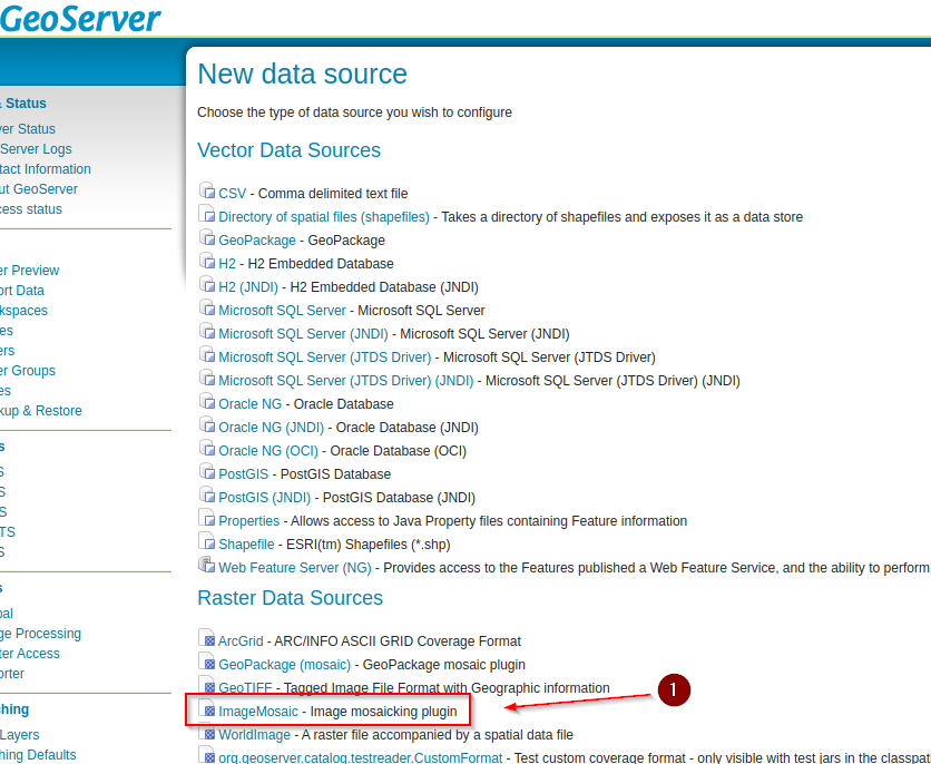
- Select `ImageMosaic` form the list of the available `Raster Data Sources`
- Provide the following inputs on the `ImageMosaic` form
* **Name**: `Aerial`
* **Title**: `Aerial`
* **URL***: `file:/opt/data/sample_data/user_data/aerial`
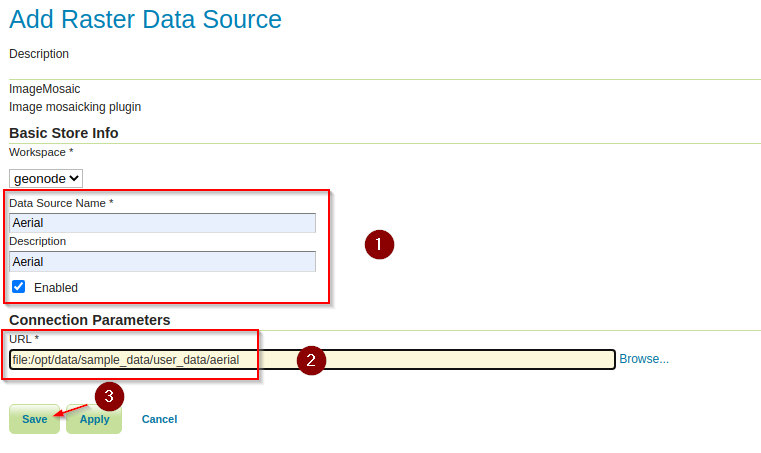
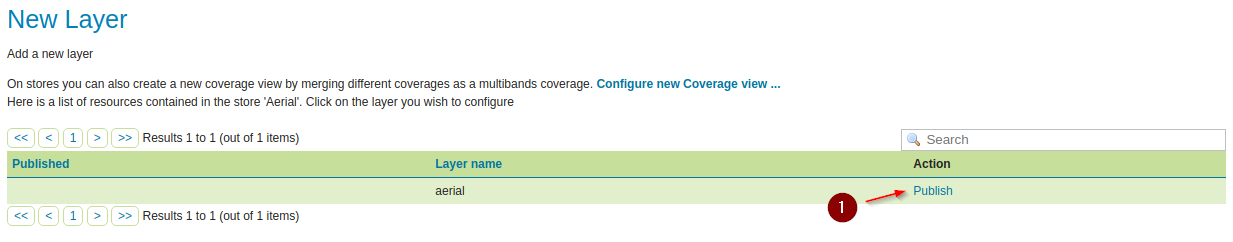
- On the next windows, click on `Publish` and `Save` the layer
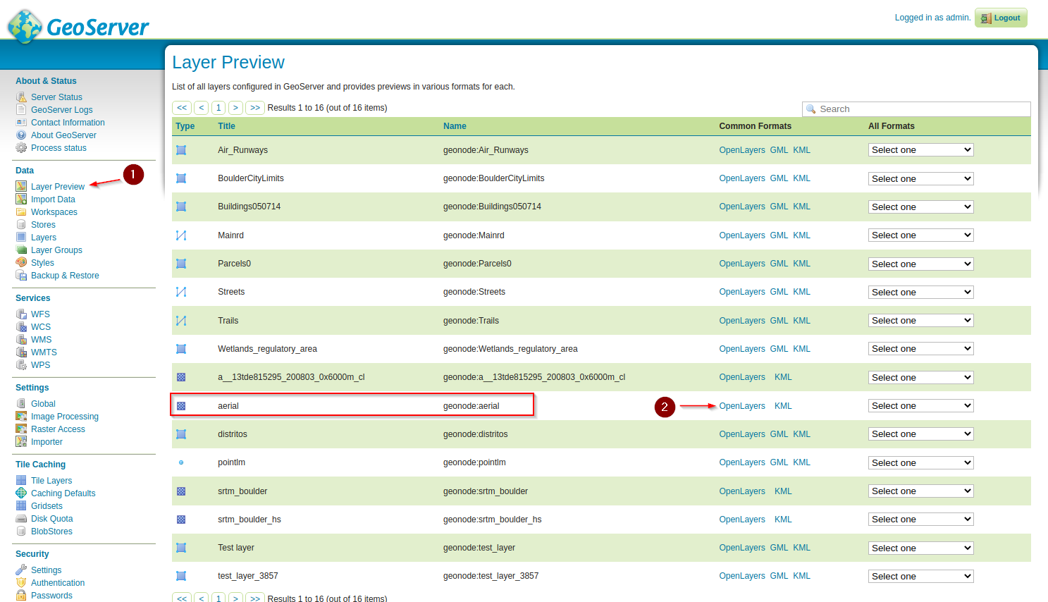
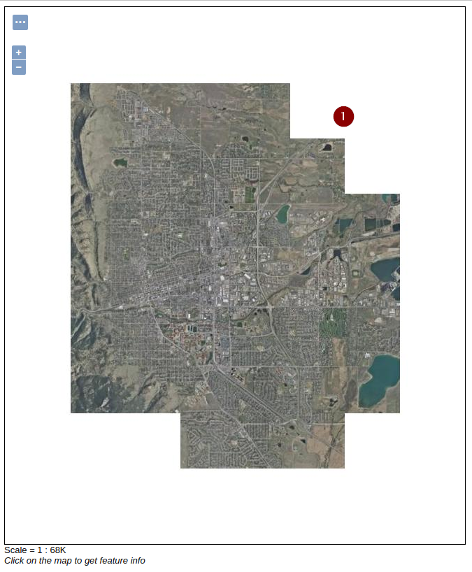
- Move to the GeoServer `Layer Preview` section and open the `OpenLayers` preview for the `Aeriel` layer
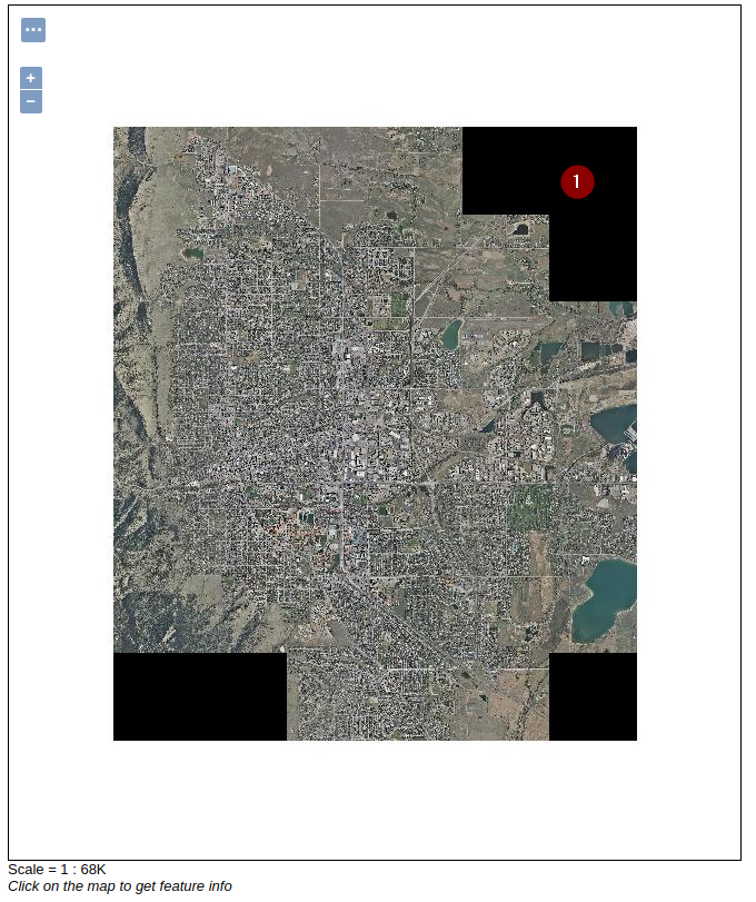
- We will suddenly notice two issues mainly:
1. The load, pan and zoom is _slow_
2. There are some _black_ tiles filling the bounding box
### Optimizing an Image Mosaic
- Open a `terminal` and move to the folder `/opt/data/sample_data/user_data`; change the `write` permissions of the folder named `optimized` in order to allow the user to modify it
```shell
cd /opt/data/sample_data/user_data
sudo chmod -Rf 777 optimized
```
- Move to `optimized` and delete the files `optimized.properties` and `sample_image.dat`
```shell
cd optimized
rm optimized.properties sample_image.dat
```
- Create or edit a file named `indexer.properties` with the following contents
```shell
vim indexer.properties
```
```ini
Caching=false
Schema=*the_geom:Polygon,location:String
```
- Create or edit a file named `datastore.properties` with the following contents
```shell
vim datastore.properties
```
```ini
SPI=org.geotools.data.postgis.PostgisNGDataStoreFactory
host=localhost
port=5432
database=geonode_data
schema=public
user=geonode
passwd=geonode
Loose\ bbox=true
Estimated\ extends=false
validate\ connections=true
Connection\ timeout=10
preparedStatements=true
create\ database\ params=WITH\ TEMPLATE\=postgis20
```
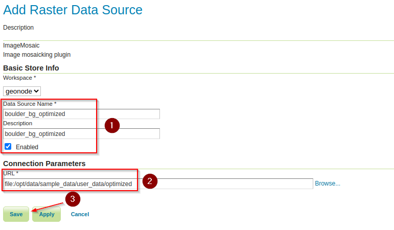
- Add a new `ImageMosaic Data Source` like we already done before and provide the following parameters
- Provide the following inputs on the `ImageMosaic` form
* **Name**: `boulder_bg_optimized`
* **Title**: `boulder_bg_optimized`
* **URL***: `file:/opt/data/sample_data/user_data/optimized`
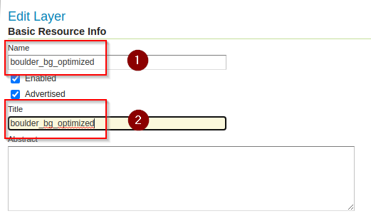
- On the next windows, click on `Publish`, **change the name and title to** `boulder_bg_optimized` and `Save` the layer
- Open the GeoServer `Layer Preview` and zoom/pan around, notice how faster is now the mosaic...
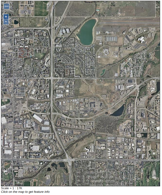
_The black tiles are still present._
- Let's customize the mosaic options in order to improve the quality and remove the black tiles.
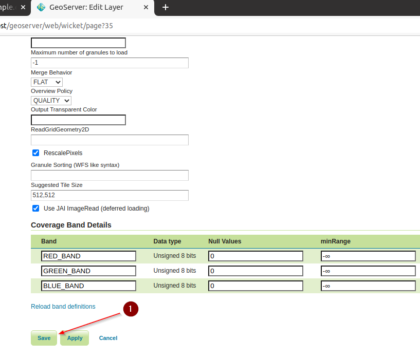
- Customize the `ImageMosaic` properties. Set the `OutputTransparentColor` to the value `000000` (Which is the `Black` color). Click on `Save` when done.
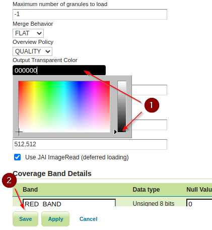
- Open the GeoServer `Layer Preview`, **clear the browser image cache** and zoom/pan around, notice the black tiles now gone
## Image Mosaic Options
There are plenty of options that can be tweaked in order to further optimize an `ImageMosaic`.
* **Accurate resolution computation**: If `true`, computes the resolution of the granules in 9 points, the corners of the requested area and the middle points and take the better one. This will provide better results for cases where there is a lot more deformation on a subregion (top/bottom/sides) of the requested bbox with respect to others. Otherwise, compute the resolution using a basic affine scale transform.
* **AllowMultithreading**: If `true`, enables tiles multithreading loading. This allows to perform parallelized loading of the granules that compose the mosaic.
* **BackgroundValues**: Sets the value of the mosaic `background`. Depending on the nature of the mosaic it is wise to set a value for the `no data` area (usually `-9999`). This value is _repeated on all the mosaic bands_.
* **Bands**: a comma separated list of band indexes that allows to expose only a particular subset of bands out of a multiband source. Normally not configured by hand, but driven by `SLD` styling instead.
* **ExcessGranuleRemoval**: An option that should be enabled when using _scattered and deeply overlapping images_. By default the image mosaic will try to mosaic toghether all images in the requested area, even if some are behind and won’t show up in the final image. With excess granule removal the system will use the image footprint to determine which granules actually contribute pixels to the output, and will end up performing the image processing only on those actually contributing. Best used along with footprints and sorting (to control which images actually stay on top). Possible values are `NONE` or `ROI` (_Region Of Interest_).
* **Filter**: Filters granules based on attributes from the input coverage.
* **Footprint Behavior**: Sets the behavior of the regions of a granule that are _outside_ of the granule footprint. Can be `None` (_Ignore the footprint_), `Cut` (_Remove regions outside the footprint from the image. Does not add an alpha channel_), or `Transparent` (_Make regions outside the footprint completely transparent. Will add an alpha channel if one is not already present_). Defaults to `None`.
* **InputTransparentColor**: Sets the transparent color for the granules prior to mosaicking them in order to control the superimposition process between them. When GeoServer composes the granules to satisfy the user request, some of them can overlap some others, therefore, setting this parameter with the opportune color avoids the overlap of no data areas between granules.
* **MaxAllowedTiles**: Sets the maximum number of the tiles that can be load simultaneously for a request. In case of a large mosaic this parameter should be opportunely set to not saturating the server with too many granules loaded at the same time.
* **MergeBehavior**: Merging behaviour for the various granules of the mosaic that GeoServer will produce. This parameter controls whether we want to merge in a single mosaic or stack all the bands into the final mosaic.
* **OVERVIEW_POLICY**: Policy used to select the best matching overview for a given target output resolution. Possible values are `QUALITY` (pick an overview with a higher resolution and downsample), `NEAREST` (pick the one with the closest resolution), `SPEED` (pick the closest one with lower resolution) and `IGNORE` (do not use overviews).
* **OutputTransparentColor**: Sets the transparent color for the created mosaic.
* **SORTING**: Allows to specify the time order of the obtained granules set. Valid values are `DESC` (descending) or `ASC` (ascending). Note that it works just by using `DBMS` as indexes.
* **SUGGESTED_TILE_SIZE**: Controls the tile size of the input granules as well as the tile size of the output mosaic. It consists of two positive integers separated by a comma, like `512,512`.
* **USE_JAI_IMAGEREAD**: If `true`, GeoServer will make use of `JAI ImageRead` operation and its deferred loading mechanism to load granules; if `false`, GeoServer will perform direct `ImageIO` read calls which will result in immediate loading.
## Introduction To Processing With GDAL Utilities
It’s a common practice to do a preliminary analysis on the available data and, if needed, _optimize_ it, since configuring big layers without proper `pre-processing`, may result in low performance when accessing them.
The previous examples show the difference between a non-optimized and an optimized mosaic, i.e. mosaics with pre-processed `GeoTIFF` granules or nor.
In this section, instructions about how to do data optimization will be provided by introducing some of the `GDAL Utilities`.
### gdalinfo
This utility allows to get several info from the `GDAL` library, for instance, specific `Driver` capabilities and input `Layers/Files` properties.
#### gdalinfo - Getting Drivers Capabilities
Being `GeoTIFF` a widely adopted geospatial format, it’s useful to get information about the `GDAL GeoTIFF’s Driver` capabilities using the command
```shell
gdalinfo --format GTIFF
```
```shell
Format Details:
Short Name: GTiff
Long Name: GeoTIFF
Supports: Raster
Extensions: tif tiff
Mime Type: image/tiff
Help Topic: drivers/raster/gtiff.html
Supports: Sublayers
Supports: Open() - Open existing layer.
Supports: Create() - Create writable layer.
Supports: CreateCopy() - Create layer by copying another.
Supports: Virtual IO - eg. /vsimem/
Creation Datatypes: Byte UInt16 Int16 UInt32 Int32 Float32 Float64 CInt16 CInt32 CFloat32 CFloat64
Other metadata items:
LIBGEOTIFF=1700
LIBTIFF=LIBTIFF, Version 4.1.0
Copyright (c) 1988-1996 Sam Leffler
Copyright (c) 1991-1996 Silicon Graphics, Inc.
```
From the list of create options above, it's possible to determine the main `GeoTIFF Driver`'s writing capabilities:
* `COMPRESS`: customize the compression to be used when writing output data
* `JPEG_QUALITY`: specify a quality factor to be used by the `JPEG` compression
* `TILED`: When set to `YES` it allows to tiled output data
* `BLOCKXSIZE, BLOCKYZISE`: Specify the Tile dimension width and Tile dimension height
* `PHOTOMETRIC`: Specify the photometric interpretation of the data
* `PROFILE`: Specify the `GeoTIFF` profile to be used (some profiles only support a minimal set of `TIFF Tags` while some others provide a wider range of `Tags`)
* `BIGTIFF`: Specify when to write data as `BigTIFF` (A `TIFF` format which allows to break the `4GB Offset` boundary)
#### gdalinfo - Getting Layer/File Properties
The following instructions allow you to get information about the sample layer previously configured in GeoServer
```shell
cd /opt/data/sample_data/user_data/aerial
```
```shell
gdalinfo 13tde815295_200803_0x6000m_cl.tif
```
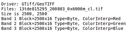
_Part of the gdalinfo output on a sample layer._
* **Block**: It represents the internal tiling. Notice that the sample layer has tiles made of 16 rows having width equals to the full image width.
* **Overviews**: It provides information about the underlying overviews. Notice that the sample layer doesn’t have overviews since the Overviews property is totally missing from the gdalinfo output.
### gdal_translate
This utility allows to convert a layer to a different format by allowing a wide set of parameters to customize the conversion.
Running the command
```shell
gdal_translate
```
allows to get the list of supported parameters as well as the supported output formats
```shell
Usage: gdal_translate [--help-general]
[-ot {Byte/Int16/UInt16/UInt32/Int32/Float32/Float64/
CInt16/CInt32/CFloat32/CFloat64}] [-strict]
[-of format] [-b band] [-mask band] [-expand {gray|rgb|rgba}]
[-outsize xsize[%] ysize[%]]
[- unscale] [-scale [src_min src_max [dst_min dst_max]]]
[-srcwin xoff yoff xsize ysize] [-projwin ulx uly lrx lry]
[-a_srs srs_def] [-a_ullr ulx uly lrx lry] [-a_nodata value]
[-gcp pixel line easting northing [elevation]]*
[-mo "META-TAG=VALUE"]* [-q] [-sds]
[-co "NAME=VALUE"]* [-stats]
src_layer dst_layer
```
The meaning of the main parameters is summarized below
* `-ot`: allows to specify the output datatype (Make sure that the specified datatype is contained in the Creation Datatypes list of the Writing driver)
* `-of`: specify the desired output format (GTIFF is the default value)
* `-b`: allows to specify an input band to be written in the output file. (Use multiple -b option to specify more bands)
* `-mask`: allows to specify an input band to be write an output layer mask band.
* `-expand`: allows to expose a layer with 1 band with a color table as a layer with 3 (rgb) or 4 (rgba) bands. The (gray) value allows to expand a layer with a color table containing only gray levels to a gray indexed layer.
* `-outsize`: allows to set the size of the output file in terms of pixels and lines unless the % sign is attached in which case it’s as a fraction of the input image size.
* `-unscale`: allows to apply the scale/offset metadata for the bands to convert from scaled values to unscaled ones.
* `-scale`: allows to rescale the input pixels values from the range src_min to src_max to the range dst_min to dst_max. (If omitted the output range is 0 to 255. If omitted the input range is automatically computed from the source data).
* `-srcwin`: allows to select a subwindow from the source image in terms of xoffset, yoffset, width and height
* `-projwin`: allows to select a subwindow from the source image by specifying the corners given in georeferenced coordinates.
* `-a_srs`: allows to override the projection for the output file. The srs_def may be any of the usual GDAL/OGR forms, complete WKT, PROJ.4, EPSG:n or a file containing the WKT.
* `-a_ullr`: allows to assign/override the georeferenced bounds of the output file.
* `-a_nodata`: allows to assign a specified nodata value to output bands.
* `-co`: allows to set a creation option in the form “NAME=VALUE” to the output format driver. (Multiple -co options may be listed.)
* `-stats`: allows to get statistics (min, max, mean, stdDev) for each band
* `src_layer`: is the source layer name. It can be either file name, URL of data source or sublayer name for multi*-layer files.
* `dst_layer`: is the destination file name.
#### gdal_translate - Tiling the sample layer
The following steps provide instructions to tile the sample layer previously configured in GeoServer, by using the GeoTiff driver.
- Move to the parent folder `/opt/data/sample_data/user_data`
```shell
cd /opt/data/sample_data/user_data
```
- Convert the input sample data to an output file having tiling set to `512x512` (the compression parameters are explained in).
```shell
gdal_translate -co "TILED=YES" -co "BLOCKXSIZE=512" -co "BLOCKYSIZE=512" -co "COMPRESS=JPEG" -co "PHOTOMETRIC=YCBCR" -co "QUALITY=85" aerial/13tde815295_200803_0x6000m_cl.tif retiled/13tde815295_200803_0x6000m_cl.tif
```
- Check that the output layer has successfully been tiled, by running the command
```shell
gdalinfo retiled/13tde815295_200803_0x6000m_cl.tif
```
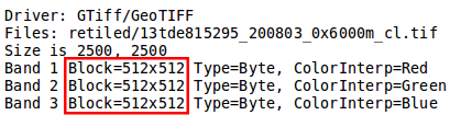
_Part of the gdalinfo output on the tiled layer. Notice the Block value now is 512x512._
### gdaladdo
This utility allows to add overviews to a layer. The following steps provide instructions to add overviews to the tiled sample layer.
Running the command
```shell
gdaladdo
```
allows to get the list of supported parameters
```shell
Usage: gdaladdo [-r {nearest,average,gauss,average_mp,average_magphase,mode}]
[-ro] [--help-general] filename levels
```
The meaning of the main parameters is summarized below
* `-r`: allows to specify the resampling algorithm (Nearest is the default value)
* `-ro`: allows to open the layer in read-only mode, in order to generate external overview (for GeoTIFF especially)
* `filename`: represents the file to build overviews for.
* `levels`: allows to specify a list of overview levels to build.
#### gdaladdo - Adding overviews to the sample layer
- Move to the `retiled` folder
```shell
cd retiled
```
- Run the `gdaladdo` command as follows
```shell
gdaladdo -r average --config COMPRESS_OVERVIEW JPEG --config PHOTOMETRIC_OVERVIEW YCBCR --config JPEG_QUALITY_OVERVIEW 85 13tde815295_200803_0x6000m_cl.tif 2 4 8 16 32
```
- Check that the overviews have been added to the layer, by running the command
```shell
gdalinfo 13tde815295_200803_0x6000m_cl.tif
```
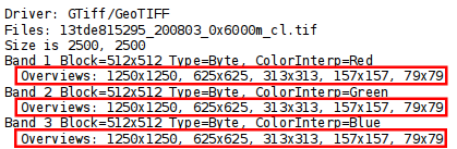
_Part of the gdalinfo output on the tiled layer with overviews. Notice the Overviews properties._
#### Process in Bulk
Instead of manually repeating these 2 steps (retile + add overviews) for each file, we can invoke a few commands to get it automated.
```shell
cd /opt/data/sample_data/user_data/aerial
```
```shell
for i in `find *.tif`; do gdal_translate -CO "TILED=YES" -CO "BLOCKXSIZE=512" -CO "BLOCKYSIZE=512" -co "COMPRESS=JPEG" -co "PHOTOMETRIC=YCBCR" -co "QUALITY=85" $i ../optimized/$i; gdaladdo -r average --config COMPRESS_OVERVIEW JPEG --config PHOTOMETRIC_OVERVIEW YCBCR --config JPEG_QUALITY_OVERVIEW 85 ../optimized/$i 2 4 8 16 32; done
```
You should see a list of run like this
```python
...
Input file size is 2500, 2500
0...10...20...30...40...50...60...70...80...90...100 - done.
0...10...20...30...40...50...60...70...80...90...100 - done.
Input file size is 2500, 2500
0...10...20...30...40...50...60...70...80...90...100 - done.
0...10...20...30...40...50...60...70...80...90...100 - done.
Input file size is 2500, 2500
0...10...20...30...40...50...60...70...80...90...100 - done.
0...10...20...30...40...50...60...70...80...90...100 - done.
...
```
At this point optimized layers have been prepared and they are ready to be served by GeoServer as an `ImageMosaic`.
### gdalwarp
This utility allows to warp and reproject a layer. The following steps provide instructions to reproject the aerial layer (which has `EPSG:26913` coordinate reference system) to `WGS84` (`EPSG:4326`).
Running the command
```shell
gdalwarp
```
allows to get the list of supported parameters
```shell
Usage: gdalwarp [--help-general] [--formats]
[-s_srs srs_def] [-t_srs srs_def] [-to "NAME=VALUE"]
[-order n | -tps | -rpc | -geoloc] [-et err_threshold]
[-refine_gcps tolerance [minimum_gcps]]
[-te xmin ymin xmax ymax] [-tr xres yres] [-tap] [-ts width height]
[-wo "NAME=VALUE"] [-ot Byte/Int16/...] [-wt Byte/Int16]
[-srcnodata "value [value...]"] [-dstnodata "value [value...]"] -dstalpha
[-r resampling_method] [-wm memory_in_mb] [-multi] [-q]
[-cutline datasource] [-cl layer] [-cwhere expression]
[-csql statement] [-cblend dist_in_pixels] [-crop_to_cutline]
[-of format] [-co "NAME=VALUE"]* [-overwrite]
srcfile* dstfile
```
The meaning of the main parameters is summarized below
* `-s_srs`: allows to specify the source coordinate reference system
* `-t_srs`: allows to specify the target coordinate reference system
* `-te`: allows to set georeferenced extents (expressed in target CRS) of the output
* `-tr`: allows to specify the output resolution (expressed in target georeferenced units)
* `-ts`: allows to specify the output size in pixel and lines.
* `-r`: allows to specify the resampling method (one of `near`, `bilinear`, `cubic`, `cubicspline` and `lanczos`)
* `-srcnodata`: allows to specify band values to be excluded from interpolation.
* `-dstnodata`: allows to specify nodata values on output file.
* `-wm`: allows to specify the amount of memory (expressed in megabytes) used by the warping API for caching.
#### gdalwarp - Reprojecting sample layer to WGS84
- Move to the `/opt/data/sample_data/user_data/retiled` folder
```shell
cd /opt/data/sample_data/user_data/retiled
```
- Run the `gdalwarp` command
```shell
gdalwarp -t_srs "EPSG:4326" -co "TILED=YES" 13tde815295_200803_0x6000m_cl.tif 13tde815295_200803_0x6000m_cl_warped.tif
```
- Check that reprojection has been successfull, by running the command
```shell
gdalinfo 13tde815295_200803_0x6000m_cl_warped.tif
```
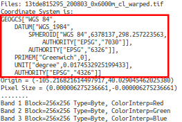
_Part of the gdalinfo output on the warped layer. Notice the updated Coordinate System property._
### Further Reading about GDAL
```shell
https://geoserver.geo-solutions.it/educational/en/raster_data/advanced_gdal/index.html
```
## Publish the Optimized Mosaic on GeoNode
- Activate the `geonode` virtual env and move to `/opt/geonode`
- Run the `updatelayers` management command as follows
```shell
./manage_local.sh updatelayers --skip-geonode-registered -u test_user1 -w geonode -f boulder_bg_optimized
```
- Verify the new layer has been succesfully created on GeoNode
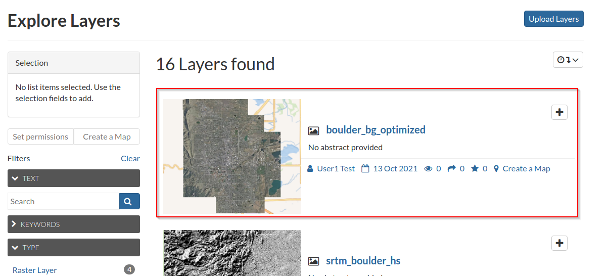
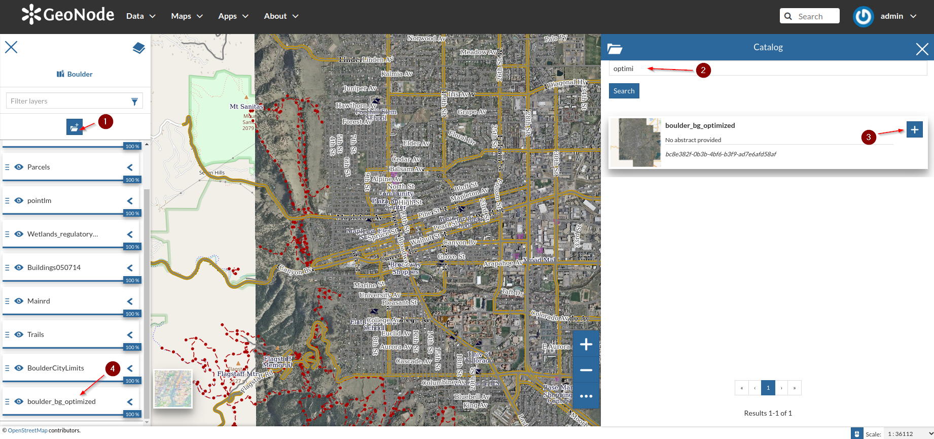
- Add the new layer to the `Boulder` map, and drag it to the bottom
#### [Next Section: Optimizing, publishing and styling Vector data](OPTIMIZE_VECTOR.md)